Most guides to backtesting py code teach the same twenty lines. Subclass Strategy, precompute in init, act in next, print the stats table. Then they stop, and what they rarely say is that the library's defaults all lean one way: toward a nicer equity curve than you'd get in a live account.
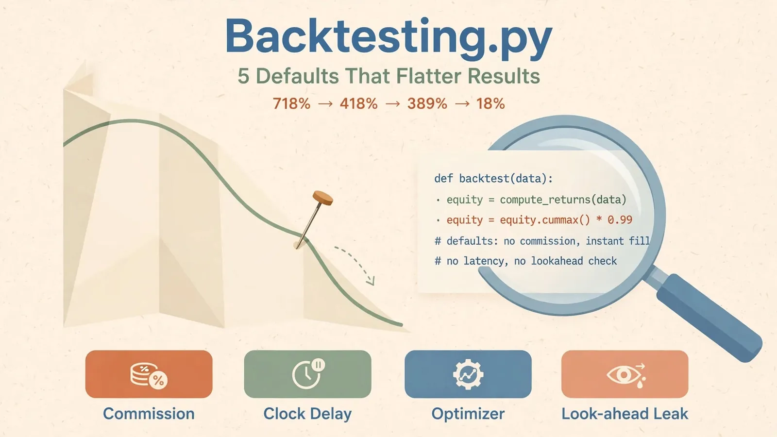
So we ran the numbers instead of describing them, using the same strategy and the same data with one default changed at a time. The headline: a moving-average crossover that shows a 718% return out of the box drops to 418% once you add a modest commission and spread, to 389% if you act one bar later, and to an 18% return on data the optimizer never saw. And a single wrong line in an indicator turned it into a 36,053% return with an 83% win rate. None of that triggered a single warning from the engine.
What does backtesting mean in this library?
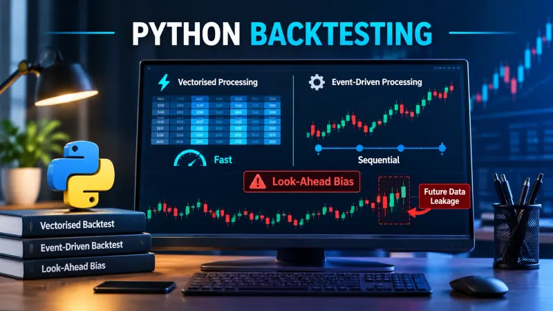
If you're asking what does backtesting mean at all, start with our plain-English definition of backtesting. In short, it means replaying a fixed rule over historical prices and recording what the rule would have done. Backtesting.py is one small, readable Python engine for doing that on a single instrument, bar by bar. It's event-driven, which means next() gets called once per bar and you can only see data up to that bar from inside it. That's a real safety feature compared with fully vectorised tools like the ones in our vectorbt glossary entry. It's also why people trust its output more than they should.
Our test setup and methodology
Everything below was run on 17 November 2026. Here's the full methodology so you can repeat it:
- Library: backtesting.py 0.6.6, installed from PyPI that day. Python 3.14.4, pandas 3.1.1.
- Data: the
GOOGdaily fixture that ships inside the package (backtesting.test.GOOG). It holds 2,148 bars from 19 August 2004 to 1 March 2013. - Strategy: the library's own example, a 10/20 simple moving-average crossover that flips long and short. Starting cash $10,000.
- Rule: change one setting per run and keep everything else fixed.
We picked the bundled data and the stock example on purpose. Anyone can reproduce our numbers in five minutes, and nobody can say we tuned the strategy to make a point. This is a teaching sample of one stock over 8.5 years, not evidence that the strategy works.
The working example (correct, but not the point)
pip install backtesting
from backtesting import Backtest, Strategy
from backtesting.lib import crossover
from backtesting.test import SMA, GOOG # columns: Open, High, Low, Close, Volume
class SmaCross(Strategy):
 n1 = 10
 n2 = 20
 def init(self):
 # precompute once; self.I() registers the indicator for plotting
 self.s1 = self.I(SMA, self.data.Close, self.n1)
 self.s2 = self.I(SMA, self.data.Close, self.n2)
 def next(self):
 # runs once per bar, sees only data up to this bar
 if crossover(self.s1, self.s2):
 self.position.close(); self.buy()
 elif crossover(self.s2, self.s1):
 self.position.close(); self.sell()
stats = Backtest(GOOG, SmaCross, cash=10_000).run()
print(stats)
Your own DataFrame needs a DatetimeIndex and capitalised Open, High, Low, Close columns (Volume is optional). Lower-case names are the most common first error we've seen. With default settings, this prints a 718.12% return, a Sharpe ratio of 0.72, a maximum drawdown of -32.79%, 93 trades, a 54.84% win rate and a profit factor of 2.27. Buy-and-hold over the same window returned 607.37%. It looks like a winner on paper, so now let's take it apart one default at a time.
Default one: the fill price you were given
Per the official backtesting.py documentation, a market order placed in next() fills at the next bar's open by default. You can switch that to the current bar's close with trade_on_close=True. Either way, the fill is exact, with no partial fill, no queue and no gap risk beyond what the open price already shows.
That's a reasonable approximation for a slow daily strategy, but a poor one for any rule whose edge lives inside the bar, or in the minutes after a signal, when real orders fight for the same price. We measured how sensitive this strategy is to the timing alone:
| Fill assumption | Return | Sharpe | Max DD | Win rate | Profit factor |
|---|---|---|---|---|---|
| Default: next bar's open | 718.12% | 0.72 | -32.79% | 54.84% | 2.27 |
trade_on_close=True | 629.60% | 0.67 | -33.30% | 50.54% | 2.20 |
| Signal acted on one bar later | 388.97% | 0.55 | -43.64% | 50.54% | 1.86 |
In the last row, waiting one extra day cut the return by almost half and pushed the drawdown from -32.79% to -43.64%. Notice too that filling at the close did worse here than filling at the next open. The direction of fill bias isn't fixed, because it depends on the strategy. What's fixed is that a result which collapses when you shift it by one bar was never strong. Run that delay test on every strategy before you believe any of its numbers.
Default two: trading costs start at zero
Commission defaults to 0, and in 0.6.x there's also a spread argument, and it defaults to 0 as well. That means every trade in the default run is free. For a strategy with 93 round trips over 8.5 years, that matters less than it would for a day-trading rule, and it still matters a lot:
| Cost setting | Return | Sharpe | Max DD | Profit factor |
|---|---|---|---|---|
| Default: no costs | 718.12% | 0.72 | -32.79% | 2.27 |
commission=0.002 (0.2% per fill) | 462.64% | 0.60 | -33.93% | 1.99 |
commission=0.002, spread=0.001 | 418.16% | 0.57 | -34.52% | 1.93 |
A 0.2% fee per fill plus a 0.1% spread took 300 percentage points off the return. More to the point, the strategy went from beating buy-and-hold (607.37%) to trailing it badly. The code and data were identical, and the only change was admitting that trades cost money.
Pick a cost that matches your broker and instrument, then add a safety margin on top; if the edge disappears at twice your expected transaction cost, treat it as fragile. We go deeper on this in our piece on why backtests and live trading drift apart.
Default three: one instrument, no portfolio
Backtesting.py runs one price series at a time. There's no shared cash pool across symbols, no position limit across a book and no correlation effect. If you test the same rule on 20 stocks one by one and add up the results, you've built a portfolio the engine never simulated. In practice, those 20 positions would compete for the same capital and, during correlated selloffs, frequently lose money on the same day.
There's a quieter problem too, because one stock is a sample of one. Our GOOG run covers a single company through a single long bull phase and the 2008 crash. A strategy that worked there tells you about GOOG from 2004 to 2013, and not much about anything else. If you need multi-asset logic, use a portfolio engine, or at least test the rule on many symbols and look at the spread of outcomes rather than the average.
Default four: the optimizer grades its own homework
Backtest.optimize() is a grid search (it can also use random or model-based search). It tries every parameter combination you give it and returns the one with the highest score. That's useful for exploring, but it becomes a problem when the top cell is quoted as "the strategy's Sharpe ratio", because it was picked using the same data it's being scored on.
We ran a grid of 33 valid combinations: fast average 5 to 30, slow average 10 to 70, fast always shorter than slow, ranked on Sharpe ratio across the full sample.
stats, heatmap = bt.optimize(
 n1=range(5, 31, 5),
 n2=range(10, 71, 10),
 constraint=lambda p: p.n1 < p.n2,
 maximize='Sharpe Ratio',
 return_heatmap=True,
)
Sharpe ratios across the grid ran from -0.29 to 0.72, with a median of 0.22. The winning cell was 10/20, the exact pair the documentation uses. That's a coincidence worth noticing: did the example's authors pick 10/20 because it looks good on this fixture? We don't know, and that's exactly the point here. When the demo parameters are also the grid's best on the demo data, you can't tell a strong rule from a lucky one.
So we did what makes a number reportable and split the data: train on 2004 to 2010 (1,605 bars), test on January 2011 to March 2013 (543 bars). The optimizer only saw the training set.
| Sample | Best params | Return | Sharpe | Profit factor | Buy & hold |
|---|---|---|---|---|---|
| Train, 2004 to 2010 | 10/20 | 566.47% | 0.80 | 2.58 | 421.16% |
| Holdout, 2011 to 2013 | 10/20 (frozen) | 18.05% | 0.31 | 1.19 | 34.28% |
The Sharpe ratio fell from 0.80 to 0.31 and the strategy lost to buy-and-hold on unseen data. The holdout figure is the honest one, and the only one worth quoting. Our overfitting guide explains why this gap appears, and walk-forward testing is the next step up: repeat the train-then-test split across several rolling windows instead of just once.
One practical note from our own run: on Python 3.14, optimize() crashed with a RuntimeError about starting a new process before bootstrapping had finished. Python 3.14 changed the default way Linux starts worker processes, as the Python multiprocessing documentation describes, and the engine uses a process pool for grid search. Wrapping the script body in if __name__ == '__main__': fixed it. Plain run() calls worked fine either way, so you'll only hit this once you start optimizing.
The data layer nobody checks
The engine checks that your columns exist, but it doesn't check whether the prices make sense. Three data problems each produce a specific wrong answer:
Missing bars. A gap of 5 days in a daily series looks like one bar to the engine. Moving averages stretch over a longer real period than you think, and a 20-bar lookback silently becomes 24 calendar days of trading. Count the bars per year before you start, since a US stock should show roughly 252.
Unadjusted splits. A 2-for-1 split in raw prices shows up as a 50% overnight crash, which a short-side rule will happily "catch" and record as an enormous fictitious win. Use split-adjusted data, and scan for any single-bar move larger than 30% before trusting a result.
Timezone mismatches. If your index is in UTC and the exchange trades in New York time, intraday bars can land on the wrong date. Daily resampling then mixes two sessions into one bar. Convert the index with pandas' tz_convert before you resample, not after.
None of these throws an error, and the output just quietly changes.
Which stats are fragile?
The stats object prints about 30 rows. Two of them get quoted most and deserve the least trust on a small sample.
Sharpe ratio on short history. Our holdout covered 543 bars and gave 0.31. The training set gave 0.80. Neither number has narrow error bars at these sample lengths. A Sharpe ratio built on two years of daily data can swing by several tenths from one random period to the next. Read our Sharpe ratio explainer before quoting one.
Max drawdown on few trades. With 23 trades in the holdout, the worst drawdown you saw is one draw from a wide range. A live account will likely see a deeper one at some point, and you should size for that. The profit factor has the same weakness, and we've written about how profit factor makes weak strategies look good.
More useful rows: # Trades (is the sample big enough?), Exposure Time [%] (how often are you even in the market?) and Buy & Hold Return [%] (did you beat doing nothing?).
Default five: look-ahead inside your own indicator
This is the one most backtesting py tutorials skip, and it's the most dangerous. The engine protects you inside next(), where you can't read tomorrow's bar. But indicators are calculated once in init(), over the whole array at once. If your own function peeks forward, the engine has no way to know, because it checks the API and not your arithmetic.
We swapped one line so that the fast average became a centred rolling mean, which is a common smoothing choice in data analysis:
import pandas as pd
def centred(x, n):
 # centre=True uses n/2 FUTURE bars - look-ahead
 return pd.Series(x).rolling(n, center=True).mean().values
class Leaky(SmaCross):
 def init(self):
 self.s1 = self.I(centred, self.data.Close, self.n1)
 self.s2 = self.I(SMA, self.data.Close, self.n2)
The result: a 36,053.25% return, Sharpe 1.68, an 83.10% win rate and a profit factor of 27.30, against 718.12% for the honest version. The engine gave no warning and no error. Per the pandas rolling documentation, center=True sets the label at the centre of the window, so each value includes bars that haven't happened yet. Other common ways in: .shift(-1), a filter that runs forwards and backwards over the series, normalising by the whole series' max or mean, and reading the high or low of the bar you're acting on as if it were known at the open.
Two checks catch almost all of it:
- The truncation test. Compute the indicator on the full series and again on the series cut off at some bar, say bar 1,000. The values at bar 1,000 must match. We found the plain SMA gave 478.786 both ways. The centred version gave 488.015 on full data and nothing at all (NaN) on the cut series, because the future bars it needed didn't exist. If any value differs, your indicator sees the future.
- The too-good test. A win rate above 75% or a profit factor above 5 on a simple trend rule is a red flag, not a discovery. Shift the signal by one bar as in default one. Honest edges shrink a bit, while leaky edges collapse.
We cover the same bug from the vectorised side in our comparison of Python backtesting libraries.
Is backtesting.py still maintained?
Don't take our word, or any tutorial's, and check it on the day you adopt it. Open the project's GitHub repository, then look at the date of the latest commit, the latest release on PyPI and how many recent issues have replies. We installed 0.6.6 from PyPI on 17 November 2026. Some older tutorials use argument names and behaviours from earlier versions, so match your code to the version you actually install.
A Python backtest and a chart indicator answer different questions
A Python backtest tells you how a fully specified rule behaved on one data file under one set of fill and cost assumptions. A chart indicator shows you a signal as each bar forms, and often repaints or confirms at the bar's close. If you move a rule from one to the other, re-check the signal timing bar by bar. A crossover that fires at the close on a chart and fills at the next open in Python is the same idea with two different P&L profiles, as our delay test showed.
Quantzee builds analytical tools for traders, not trading advice, and nothing here suggests this strategy should be traded. The aim is narrower: when your own backtest says 700%, you should know which defaults produced that number and how to strip each one out.