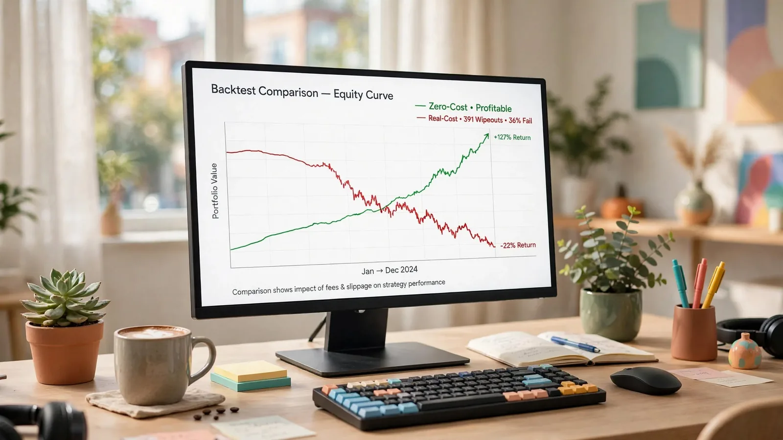
Score your grid twice before you believe any of it. Run the exact same parameter combinations once with transaction cost set to zero and once with a stated, realistic round-trip charge, then read the gap between the two columns — not either column alone. That gap is the number that decides which timeframes you are actually allowed to trade. We ran this procedure across 1,080 real-cost combinations and their 1,080 zero-cost twins, and 391 of the real-cost combinations (36%) lost the entire notional. Nothing on that losing list was a surprise once you saw where the losses clustered: the fastest charts, where trade count is highest and cost compounds hardest.
Every backtesting guide on this topic tells you to "include commissions and slippage." According to the most widely cited of them, a fast strategy "might be breakeven or negative after costs" — one sentence, no arithmetic behind it. We built the arithmetic instead. This post walks through what we found when we scored the same grid twice: the procedure, the stated cost assumptions, the headline wipeout count, where the survivors live, and what a second honest haircut — counting your tests — does to even the surviving numbers.
The Procedure: Score the Grid Twice, Never Once
The method here is not complicated, and that is the point. Take a parameter grid. Run it once with transaction cost assumed away — a zero-cost scenario that no broker, exchange or venue has ever offered — and run it again with a stated, realistic round-trip cost applied to every single trade. Label both columns. Read the real-cost column for what the setting actually did. Read the zero-cost column only to measure how much of the first column's result was signal and how much was handed over in cost.
A result reported without the cost assumption stated next to it is not a result — it's an unlabelled number that could mean anything from a durable edge to a strategy that trades itself to zero the moment a broker gets paid. We built this comparison into the full SuperTrend backtest results grid, and the paired columns are exactly what let a reader check the claim instead of trusting it.
The Grid and the Engine
The dataset behind this post is a full parameter sweep of the SuperTrend indicator. ATR period runs {7, 10, 14, 20, 30}, crossed with multiplier from 1.0 to 5.0 in steps of 0.5 — 45 combinations. That grid runs across eight timeframes from 1-minute to daily, on three instruments (BTC, Gold and Silver), in two cost scenarios: 45 × 8 × 3 × 2 = 2,160 rows. 1,080 of those rows carry transaction cost; 1,080 are at zero cost. Every single one is published — losers, wiped-out rows and winners side by side, none filtered out.
Mechanics, stated up front because they change what a number means: long/short, flip on signal, always in market, no pyramiding. Entry and exit fill at the next bar's open after the flip bar's close confirms the signal — no lookahead. The engine is vectorbt's Portfolio.from_signals, with full equity reinvested on every trade. Full reinvestment matters for what comes next: it means a losing run compounds its losses the same way a winning run compounds its gains, and a bad enough losing streak can take the account to zero.
The Cost Assumptions — Stated, Not Measured
The round-trip cost figures used in the real-cost column are stated assumptions, not measured fills, because the underlying price data carries no bid-ask spread to measure from. We want that distinction on the record every time a number is quoted from this dataset. BTC carries an assumed 15 basis points round-trip — a taker fee of roughly 0.05% per side plus an estimated 0.025% per side of slippage. Gold (XAUUSD) carries 4 basis points round-trip, for a tight institutional spot/futures spread. Silver (XAGUSD) carries 8 basis points, proportionally wider than Gold's spread. None of these three figures were measured from an actual fill; they are a conservative, stated convention applied uniformly to every trade in the grid, and the SuperTrend settings guide repeats them next to the per-instrument winner tables so a reader never has to take them on faith.
If your own broker charges more or less, the gap between your zero-cost and real-cost columns will be wider or narrower than ours — the direction of the finding (fast timeframes die, slow timeframes survive) does not change, but the exact wipeout count will move with the cost assumption. That is a feature of running the comparison this way, not a flaw: you can re-run it with your own number and see where your personal cost structure moves the line.
The Headline: 391 of 1,080 Real-Cost Combinations Wiped Out
391 of the 1,080 real-cost combinations — 36% of the grid — lost the entire notional under full reinvestment, meaning total return at or below -100%. A further 14 of the 1,080 zero-cost combinations hit the same wall even with no transaction cost applied at all, which tells you those 14 were never viable on signal quality alone; cost simply added 377 more losses on top.
Here is what that 36% figure hides if you don't look at where it clusters. Of the 391 real-cost wipeouts, every single 1-minute combination failed (135 of 135). On the 3-minute chart, 120 of 135 failed. On 5-minute, 96 of 135. On 15-minute, the number drops to 30 of 135, and on 30-minute it drops again to 10 of 135. From the 1-hour chart upward — 1h, 4h and 1d — there were zero wipeouts in the entire real-cost grid. The wipeout isn't random across the parameter space; it is a function of how fast the chart is, full stop.
One more figure worth stating plainly, because sorting this dataset by drawdown without it will mislead you. Once a run's equity reaches or crosses zero mid-test, vectorbt's drawdown percentage is computed against a near-zero equity base. It explodes to a nonsensical magnitude — the worst row in this grid reads a drawdown on the order of -1014%. That is a divide-by-near-zero artifact, not a real number. Total return percentage, floored at -100% because it matches total profit against the starting notional, is the trustworthy figure to read on a wiped-out row — never its drawdown column.
Where the Survivors Live: Nothing Fast, Everything on the 4-Hour Chart
Here is the part that should change how you choose a timeframe before you choose a setting. Far more than three combinations were profitable after real costs across this grid — 95 on Gold, 93 on Silver, and 38 on BTC, out of 360 real-cost combinations tested per instrument. But when you rank those profitable combinations and take the single best setting for each instrument, all three best-of-instrument picks land on the 4-hour chart. Not one of them is an intraday setting, and not one of them is a daily setting either.
Gold's best real-cost combination — ATR period 30, multiplier 2.5, on the 4-hour chart — returned $153,319 total profit (153.3% of notional) across 2,484 days, averaging about $62 per day, with a maximum drawdown of -25.7%, a Sharpe ratio of 1.01, across 340 trades. Silver's best — ATR period 30, multiplier 3.5, also on 4-hour — returned $1,207,727 (1,207.7%) over the same 2,484-day window, averaging roughly $486 per day, max drawdown -36.0%, Sharpe 1.50. That headline number is real, but it rests on only 191 trades, which is the sample-size caveat we come back to below before you let that return figure impress you more than it should. BTC's best — ATR period 30, multiplier 5.0, 4-hour — returned $50,090 (50.1%) over 1,026 days, averaging about $49 per day, max drawdown -53.1%, Sharpe 0.56, across 61 trades. BTC's history in this dataset starts in late 2023, so that is roughly a 2.8-year window against Gold and Silver's roughly 6.8 years — a materially shorter test on the instrument with the fewest trades of the three.
Two things to notice in that pattern beyond "4-hour won." First, the winning ATR period is 30 in all three cases — the slowest, most averaged setting in the entire {7, 10, 14, 20, 30} range tested, on the slowest chart where it was tested. Second, Gold and Silver's winning multipliers (2.5 and 3.5) sit in the middle of the range, while BTC's winner (5.0) sits at the top of it — BTC's higher volatility needed the widest band tested to avoid getting whipsawed on the same timeframe where Gold and Silver did not.
Why Cost Scales With Trade Count and the Edge Doesn't
The mechanism behind this entire pattern is simple arithmetic, which is exactly why it is so consistently reproducible across three unrelated instruments. A round-trip cost in basis points is charged once per trade, every trade, regardless of how big or small that trade's edge turned out to be. A strategy's per-trade edge — the average amount it expects to make before cost — does not scale with how many trades it takes; it is roughly constant, set by the signal and the market, not by the clock. Trade count, on the other hand, scales almost directly with how fast the chart is: a 1-minute chart on a trending instrument generates many multiples of the trade count of the same signal applied to a 4-hour chart over the same calendar period, because there are simply more bar-closes to flip on.
Multiply a fixed per-trade cost by a trade count that climbs an order of magnitude as the chart speeds up, and the cost term grows faster than the edge term that is supposed to pay for it. At some point — and in this grid, that point sits somewhere around the 15-minute to 30-minute boundary — the cost term overtakes the edge term entirely, and every trade becomes expected-value negative before the market even has a chance to move. That is why "nothing on 1m, 3m or 5m survived real cost" is not a coincidence specific to SuperTrend; it is what happens to almost any signal-flip strategy once trade count gets high enough to make transaction cost the dominant term in the equation, rather than a rounding error on top of it.
What This Does Not Prove
State the limits on the page, because a result this clean is exactly the kind that invites overreading. This dataset covers three instruments — BTC, Gold and Silver — and no equities, no forex pairs beyond those three, and no options. It tests one indicator, SuperTrend, not the five or six most common trend-following tools side by side. Silver's headline 1,207.7% return rests on 191 trades over 6.8 years; that is above the roughly 100-trade floor we'd treat as the minimum for a result to mean anything, but it is still a comparatively thin sample for a single number this large to carry. And BTC's winner is drawn from a 2.8-year window against the 6.8 years Gold and Silver get, so the three "best setting" rows are not apples-to-apples in how much market history backs each one.
None of that invalidates the core finding — the clustering of wipeouts on fast timeframes and the absence of any fast-chart survivor after real cost is consistent and large enough (391 wipeouts, zero survivors under an hour) that it is not a sampling artifact. But the specific dollar figures attached to the three per-instrument winners deserve the caveats above before you treat any one of them as a number you could expect to repeat.
The Second Honest Haircut: Counting Your Tests
There is a second adjustment that belongs next to every backtest result, and it has nothing to do with transaction cost. If you score 1,080 combinations and report only the single best one, you are reporting the single strongest outcome of a 1,080-way search. That is not the expected performance of "the strategy." The more settings you test, the more likely one of them looks good purely from noise. A result's apparent significance needs to be discounted for how many chances it had to appear strong by luck alone.
We have measured exactly this discount on a separate internal grid: 396 effective tests carried a multiple-testing haircut factor of 3.4587, meaning a raw result that looked striking before the adjustment needed to be more than three times as strong to clear the same statistical bar once the search size was accounted for. Academic work backs this up. A National Bureau of Economic Research working paper on backtesting strategies built from multiple signals finds that overfitting bias from this kind of search "severely exacerbates" the ordinary multiple-testing bias that shows up whenever a researcher considers more results than they present. The same dynamic applies to a 1,080-cell parameter grid. The U.S. Securities and Exchange Commission's investor-education glossary defines backtesting in exactly these terms: a historical simulation used to estimate how a strategy would have performed. That distinction matters because a backtest's headline number, read without accounting for how large a search produced it, is one of the most common ways retail traders mistake a lucky draw for an edge.
A reader who scores 1,080 combinations in a grid like ours and reports the single best cell — Silver at 1,207.7% on a 191-trade sample — is reporting the result of the search, not a verified property of the strategy. That does not make the number false. It makes it a candidate for further scrutiny, not a conclusion.
The Checklist to Take With You
- State the cost assumption in basis points beside every return figure you quote — a return without its cost basis attached is not comparable to anything.
- Publish both columns. A zero-cost number by itself tells you nothing about what you would actually keep; it only becomes useful next to its real-cost twin.
- Count your tests. If you searched 1,080 combinations, the single best one needs a much higher bar to clear than a result from a single pre-specified test.
- Keep a sample-size floor near 100 trades before trusting a percentage. Fewer than that, extend the test window rather than trusting the number.
- Check the neighbouring parameter values before believing any one cell. If ATR 29/multiplier 3.4 and ATR 31/multiplier 3.6 collapse next to a winning ATR 30/multiplier 3.5, you have found a curve fit, not a setting.
- Re-run the comparison periodically. A cost assumption, an instrument's volatility regime, or a market's microstructure can all drift, and a number that is a year old deserves a fresh look before you lean on it again.
None of this is a signal to trade, and nothing above is investment advice — it is the arithmetic behind one specific indicator on three specific instruments, published so you can check it rather than take it on faith. Want to run this same zero-cost-versus-real-cost comparison on your own strategy? The backtesting glossary entry and the guide to backtesting a TradingView indicator walk through the mechanics step by step. The slippage glossary entry covers how to estimate your own cost assumption, if your broker's fee schedule doesn't translate cleanly into a round-trip basis-point figure. Two failure modes show up most often once a cost-aware backtest clears this bar. One is reading profit factor instead of the full distribution of trades — see why profit factor is the metric most likely to make a bad strategy look good. The other is a mismatch between what the backtest measured and what live trading actually delivers — see backtest-vs-live-trading mismatch.
Quantzee publishes the full 2,160-row grid, not a summary, specifically so a reader can apply their own cost assumption and their own sample-size floor to the same data instead of trusting a single quoted headline. If you build and test your own indicators, the Quantzee indicator suite is built on the same real-cost-first premise this dataset demonstrates: a setting is not a setting until it survives a round-trip cost you can name.