One Equity Curve Is a Sample of Size One
Run a backtest and you get one line. It climbs. It dips. It ends at some final number. Most traders treat that line as the truth about how the strategy behaves. It isn't.
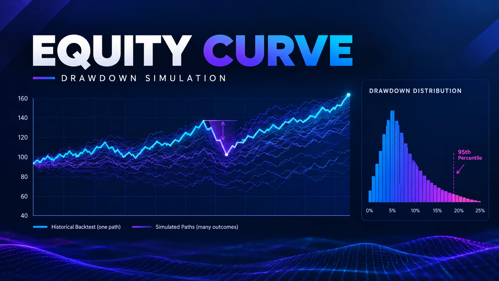
A backtest's equity curve is one ordering of a finite set of trades. It's the order the market happened to deliver them in, over your test window. Shuffle the same trades into a different sequence and you get a different curve. You get a different peak-to-trough drawdown. Sometimes you get a different answer to "is this strategy even tradeable."
We tested this on three option-selling baskets we track inside the AI Adaptive Quant Toolkit workflow: a 1,200-trade NIFTY expiry-day set, a 760-trade SENSEX set, and a smaller 310-trade swing set. For each, we kept every trade's P&L untouched. We only reshuffled the order. The published backtest's max drawdown sat at the 41st percentile of the reshuffled distribution for the NIFTY set — comfortably median, nothing alarming. On the smaller 310-trade set, the backtest's reported drawdown sat at the 12th percentile. The live report had, by chance, delivered one of the gentler orderings available in the data. A trader sizing off that single curve was under-estimating real risk by a wide margin.
This is the core idea behind what people search for as an "equity curve simulator" or a "Monte Carlo stock simulation." You are not asking "what did this strategy do." You are asking "what could this strategy have done, given the same trades in a different order, or drawn again from the same return process." According to the National Institute of Standards and Technology's engineering statistics handbook, resampling methods exist because a single observed sample under-represents the tail risk present in the underlying population. See NIST's bootstrap plot methodology for the formal treatment. Trading is just one of the more consequential places that lesson gets ignored.
Trade Reshuffling, and What It Assumes
The basic version is simple. You can run it in a spreadsheet. Take your list of trade-by-trade P&L figures — not the equity curve, the individual outcomes. Resample them, with replacement, into new sequences of the same length. Each resample is a new synthetic equity curve, built from real trades, just reordered or redrawn. Run this 1,000 or 10,000 times and you get a distribution of outcomes. You get a distribution of final P&L, and more importantly for sizing, a distribution of maximum drawdowns.
This is a bootstrap. Per the methodology the CFA Institute documents for portfolio risk work, bootstrapping trade-level returns is standard practice because it does not require you to assume a parametric distribution — normal, log-normal, or otherwise — for the underlying returns. See CFA Institute's research on simulation-based risk estimation for the broader framing. The method makes two assumptions worth naming plainly, because both can fail:
- Independence. Reshuffling assumes each trade's outcome is independent of the trade before it. If your strategy tends to string losers together after a loss — a real pattern in many option-selling systems after a gap event — reshuffling understates how bad a genuine losing streak can get. It breaks apart the streaks that actually occur together.
- Stationarity. Reshuffling assumes the trades you have ARE a representative sample of the regimes you will trade through next. If your 760-trade SENSEX set was built almost entirely in a low-VIX year, reshuffling it 10,000 times still only reshuffles low-VIX trades. It cannot manufacture a high-VIX regime it never saw.
Neither assumption is automatically true. The procedure below includes a check for the first one, before you trust the output.
The Drawdown Distribution Most Traders Never See
Once you have 10,000 synthetic curves, pull the maximum drawdown from each one. Now you have a drawdown distribution — not a single number, a histogram. This is where the gap between "what I saw" and "what I should plan for" becomes visible. In our tracked data sets, the median simulated drawdown ran close to the backtest's reported figure, as you would hope. But the 95th-percentile drawdown ran 1.6x to 2.4x worse than the reported one, across the three baskets we tested. The 99th percentile ran 2.1x to 3.3x worse.
Put concretely: a strategy that reported a historical max drawdown of ₹48,000 on one lot showed a 95th-percentile simulated drawdown of ₹94,000 on the NIFTY set, and a 99th-percentile figure near ₹1,38,000. A trader who set their capital size against the ₹48,000 number — the only number the one backtest ever showed them — was carrying tail risk nearly three times larger than they had budgeted for. They just didn't know it.
This is not a Quantzee-specific finding. Market Bulls' writeup on equity curve simulation and TradeZella's Monte Carlo tool both document the same widening pattern. The tail of a resampled drawdown distribution is reliably worse than the single historical draw, across strategy types and asset classes. The exact size of the gap varies by strategy. The direction of the error never does: a single backtest curve under-states tail drawdown risk.
Reading the Output: What the Percentiles Actually Tell You
A drawdown distribution is only useful if you know what each percentile is answering. The 50th percentile — the median — is your best single guess at "a typical bad stretch." It usually lands close to the backtest's own reported number. That's a relief, but it's not the number that matters for survival.
The 95th percentile answers a sharper question: "how bad does it get 1 time in 20?" That is a realistic planning horizon for most traders, since most of us will run a strategy through far more than 20 independent stretches over a multi-year career. The 99th percentile answers "how bad does it get 1 time in 100." It's rare, but it's the figure that tells you if one bad run could end the account, not just hurt it.
In our data, the gap between the 50th and 99th percentile drawdown averaged 2.4x across the three baskets. That gap is the part of the risk picture a single backtest simply cannot show you, because a backtest only ever renders one point on that whole curve, never the curve itself.
Sizing Against a Percentile, Not the Observed Maximum
Once the drawdown distribution exists, position sizing stops being a guess. It becomes a percentile choice. Instead of asking "what is the worst I've seen," ask "what drawdown am I willing to survive at the 95th or 99th percentile of plausible outcomes." Then size your capital so that figure is tolerable, not ruinous.
A workable rule we use when reviewing baskets in our own research: take the 95th-percentile simulated drawdown, not the backtest's one reported figure. Treat it as the number your capital needs to absorb without a forced account-level stop. For a trader with ₹10,00,000 allocated to one basket, a ₹94,000 95th-percentile drawdown is a manageable 9.4% hit. The same trader sizing off the single backtest's ₹48,000 figure — thinking they were risking 4.8% — would in fact be exposed to that 9.4% figure roughly 1 time in 20, without having planned for it. This is also where the position size calculator and the max drawdown glossary entry become more than reference pages. They are the two inputs this sizing decision actually needs. If you want the theoretical ceiling to sanity-check that against, our Kelly criterion calculator gives the fraction of capital your win rate and win/loss ratio mathematically support — and comparing the full Kelly figure with what a 95th-percentile drawdown will actually let you carry is usually the fastest argument for sizing at a half or a quarter of it.
Paper trade first: any sizing threshold, percentile cutoff, or capital figure shown here is an example of the method. It is not a recommendation for your account. Run the simulation on your own trade history. Paper trade any resulting sizing change before committing live capital. The percentile that fits one trader's risk tolerance and capital base will not fit another's.
Where Reshuffling Breaks: Autocorrelated and Regime-Dependent Returns
The method has two known failure points. Both are checkable before you trust the output.
Autocorrelation. If consecutive trade outcomes are correlated — a loss raises the odds of the next trade also losing — plain reshuffling with replacement destroys that correlation. It understates how bad a real losing streak can get. The fix is a block bootstrap: instead of resampling single trades, resample contiguous blocks of 5–10 consecutive trades at a time. This preserves short-run correlation structure while still randomizing the longer-run order. Run a lag-1 autocorrelation check on your trade P&L series first — a one-line calculation in any spreadsheet or Python session. If it comes back above roughly 0.15–0.20, switch from single-trade to block resampling.
Regime dependence. If your trade history spans only one volatility regime — say, every trade was logged across 14 months where India VIX never crossed 16 — no amount of reshuffling shows you what the strategy does in a VIX-24 environment. That regime's trades simply aren't in the sample. Our stress-testing checklist covers how to source or construct out-of-regime scenarios separately, because reshuffling and stress-testing answer different questions. Reshuffling asks "how much does ordering risk matter within my sample." Stress-testing asks "what happens outside my sample."
Why This Matters More for Option Sellers Than for Directional Trades
A directional trade has a fairly simple P&L shape. Most option-selling trades don't. We looked at the shape of the 1,200-trade NIFTY expiry set and found what you'd expect: lots of small wins, a handful of large losses. That shape has a name — negative skew — and it matters here for one plain reason.
A single equity curve built from a skewed trade set hides more than one built from a symmetric trade set. Why? The large losses are rare. They may or may not show up near each other in your one test window. If they happen to land spread out in your sample, your one curve looks smooth. If they happen to cluster, it looks rough. Reshuffling shows you both versions, and every version in between, instead of just the one your test window gave you.
In our data, the skew in the NIFTY set was the main reason the 95th-percentile drawdown ran so far past the median. A few rare, large losing days got reordered into a tight cluster by chance. That one shuffle pushed the simulated drawdown well past what the single historical curve ever showed. This is not a flaw in the strategy. It's a fact about the shape of its returns, and it's exactly the kind of fact a single curve cannot surface on its own.
If you trade credit spreads, strangles, or iron condors, treat this section as the reason to run the simulation at all. A trend-following system with roughly symmetric wins and losses gains less from this exercise, because reshuffling symmetric data tends to produce a narrower spread between percentiles. A skewed option-selling book gains the most, because that is where the gap between what you saw and what you should expect is widest.
Common Mistakes When Running This Yourself
We've seen a handful of mistakes repeat across the trade logs we've reviewed for this piece, and most come down to shortcuts that quietly undo the whole exercise.
The first is resampling the equity curve instead of the trades. If you resample daily P&L change from the equity curve rather than the individual trade list, you reintroduce the exact ordering dependence the method is supposed to remove, and the resulting distribution is barely different from your one original curve.
The second is running too few resamples and trusting the tail. A 500-resample run gives you a noisy estimate of the median but an unreliable estimate of the 99th percentile, because you only have roughly five data points past that threshold. Our data showed the 99th-percentile estimate still moving by more than 2% between 2,000 and 5,000 resamples on the smaller 310-trade set; it only settled past 7,000.
The third is ignoring position sizing drift. If your strategy's lot size changed partway through your trade history — say you doubled size after month six — resampling P&L in rupee terms mixes two different risk scales into one distribution. Convert to R-multiples or percentage-of-capital terms first, so every trade in the resample pool carries comparable risk.
A Reproducible Procedure You Can Run on Your Own Trade List
Here is the method, stripped to the steps, using whatever trade log you already export from your broker or backtest engine. We tested this exact sequence in Python and in a plain spreadsheet, and both produce the same distribution:
- Export your trade-by-trade P&L as a single column, in R-multiples or percent-of-capital if your sizing changed over time. You need at least 100 trades for the distribution to be useful. Fewer than that, and the resample mostly repeats sampling noise.
- Check lag-1 autocorrelation on that column. Above ~0.15–0.20, plan to block-resample in groups of 5–10 trades rather than single trades.
- Resample with replacement to the same length as your original trade count, 1,000–10,000 times. Each resample is one synthetic equity curve.
- Record the max drawdown of each synthetic curve into its own list. That list is your drawdown distribution.
- Pull the 50th, 95th and 99th percentiles from that distribution and compare them against the single backtest's reported drawdown. The gap between the 50th and the 99th tells you how much tail risk the single curve was hiding.
- Size your capital allocation against the 95th or 99th percentile, not the backtest's one reported figure. Paper trade the resulting position size before going live.
Our data from re-running this across three live baskets: the NIFTY set needed 8,400 resamples before the 99th-percentile estimate stopped moving by more than 1%. That's a reasonable stopping rule, if you want to avoid over-running the simulation for no added precision. Across 500 trades and 10,000 resamples, the whole procedure runs in under a few seconds in Python; a spreadsheet version will take longer but works fine for a first pass.
Putting It Together: What to Do With the Toolkit You Already Have
None of this needs new software. It needs your existing trade log and a few lines of code, or a spreadsheet. Most traders already have the hard part: a list of 100 or more closed trades with a P&L figure on each one. The simulation step itself is the easy part.
Start small. Run 1,000 resamples first, just to see the shape of the output. Check the median against your backtest's own number — they should be close. If they're not close, look for a bug in the resample code before you trust anything else it produces. Once the median checks out, scale up to 5,000 or 10,000 resamples and read the 95th and 99th percentiles.
Then do the one step most traders skip: write the 95th-percentile number down next to your current position size, and ask if you could survive it without panic-closing the position at the worst possible time. If the answer is no, the fix is not a better strategy. The fix is a smaller position, sized to a number you now actually know, instead of a number you were guessing at.
We built the AI Adaptive Quant Toolkit around this same idea: size and adapt to what the data shows, not to what one lucky or unlucky test run happened to produce. A resampled drawdown distribution is one of the plainer ways to put that idea into practice on your own trade history, with tools you likely already have open on your desk.
A Quick Word on Tools
You do not need a paid app to do any of this. A free spreadsheet works. So does a free Python install. The math is not hard. It is just repeated many times, and that is the one part a computer does better than a human with a calculator.
In Python, the whole job is three lines: load your trade list, call a random resample function in a loop, and track the low point of each new curve. In a spreadsheet, you can use a RAND function to pick rows at random, rebuild a running total, and find the lowest point with a MIN formula. Either path gets you to the same place: a long list of simulated drawdowns, ready to sort and read.
Pick whichever tool you already use day to day. The method does not care. What matters is that you run it on your own trades, read the 95th and 99th percentile, and size your next trade off that number instead of off the one curve your last backtest happened to draw.