
Free Trading Tool
Sharpe Ratio Calculator
Paste the return series you already own — one per line, comma separated, or straight out of a strategy-tester return column — and the calculator works out the mean, the dispersion and the ratio for you. Or switch to summary mode and enter the three numbers directly. Either way the periods per year question is compulsory, because that single choice moves the answer more than anything else on this page. No signup required.
One return per period. Line breaks, commas, semicolons or tabs all work, so a column pasted out of a spreadsheet or a strategy-tester export goes in as-is. Percent signs, thousands separators and parentheses-negatives are handled.
A short-dated government bill yield over the same horizon as your returns. Divided by the periods-per-year figure below to get the per-period baseline. Enter 0 to measure raw return per unit of risk instead of excess return.
Your Result
Annualised Sharpe ratio
—
Per-period ratio scaled by the square root of your periods-per-year figure.
Sharpe ratio per period
—
The unscaled figure, on whatever period your data is in.
Mean return / period
—
Std deviation (sample)
—
Observations (n)
—
Annualisation factor (√N)
—
Dispersion uses the sample standard deviation (the n−1 divisor), because a pasted series is a sample of a strategy rather than its whole population. See the convention note below for why that matters at small n.
Always paper trade first. This calculator is an analytical tool for examining a strategy's risk-adjusted return before you risk capital — it is not investment advice and does not guarantee results. A high ratio measured on a backtest is a measurement of the past, so test any system on a paper account before trading it live.
Want the definition, the threshold bands and the common mistakes instead? Read the full Sharpe ratio definition →
The Sharpe Ratio Formula, Term by Term
The sharpe ratio formula divides what a strategy earned above a risk-free baseline by how much its returns moved around. Two lines do the whole job — one for the period figure, one to put it on an annual footing:
Sharpe_period = (Rp − Rf) / σp

Sharpe_annual = Sharpe_period × √N

Rp = mean return of one period
Rf = risk-free rate over that SAME period
σp = standard deviation of the period returns
N = number of those periods in a year- Rp − Rf, the numerator. This is the part traders argue about — which baseline is fair, whether to use zero when comparing two strategies against each other, whether to subtract the rate at all on an intraday series.
- σp, the denominator. This is the part that decides the answer. Shifting the risk-free assumption by a point moves the ratio a little; halving the dispersion doubles it. It is also the term every other calculator asks you to supply, which is exactly backwards — it is the hardest number to work out by hand and the easiest one to compute from a return series.
- N, the annualisation factor. Not part of the classical formula at all, and the reason two people can compute different Sharpe ratios from the same data and both be doing the arithmetic correctly.
Which dispersion convention this page uses
The calculator uses the sample standard deviation, dividing the squared deviations by n−1 rather than n. A return series is a sample of a strategy's behaviour, not the complete population of everything it will ever do, so n−1 is the right divisor. It matters at small sample sizes and almost nowhere else: on the ten-return example below the sample convention gives a ratio of 0.3847 against 0.4055 for the population convention, a 5.4% gap. At a few hundred observations the difference disappears into the rounding. Any tool that does not say which one it used is leaving you unable to reproduce its own number.
A Sharpe Ratio Calculation You Can Check by Hand
Ten monthly returns, illustrative and simulated — not a product result and not a real account. Load them into the calculator above with the example button and every number below should match.
+2.1%
-1.4%
+3.6%
+0.8%
-2.9%
+4.2%
+1.5%
-0.6%
+2.8%
+1.9%| Step | Working | Result |
|---|---|---|
| Mean monthly return | 12.0 ÷ 10 | 1.2000% |
| Sample standard deviation | n−1 divisor, n = 10 | 2.2529% |
| Risk-free, per month | 4.00% per year ÷ 12 | 0.3333% |
| Excess return | 1.2000 − 0.3333 | 0.8667% |
| Monthly Sharpe ratio | 0.8667 ÷ 2.2529 | 0.3847 |
| Annualised at N = 12 | 0.3847 × √12 = 0.3847 × 3.4641 | 1.3326 |
The 4.00% risk-free figure is a stand-in for the arithmetic, not a current rate. Printing a live rate would date the page within a week of publishing, so substitute whatever short-dated bill yield covers the period you are measuring.
Annualising: the Part That Breaks the Number
Why it scales with √N, not N
Mean return adds up over time, so twelve monthly returns give roughly twelve times one month. Standard deviation does not: variance adds, and the standard deviation is its square root, so twelve months of dispersion is about √12 times one month's. The ratio of the two therefore grows by N / √N, which is √N. Scaling the ratio linearly by N instead of by √N is the single most common annualisation error, and it inflates a monthly figure by a factor of 3.46.
The wrong-N trap, on one series
Both numbers below come from the same ten returns above, with the same mean of 1.2000% and the same dispersion of 2.2529%. The risk-free rate is set to zero for this comparison, so that N is genuinely the only thing moving — the period ratio is 1.2000 ÷ 2.2529 = 0.5326 in both columns. Enter the series with the risk-free field at 0 and you will reproduce both figures exactly:
Annualised at N = 12 (monthly data)
1.8451
Correct — the series is monthly. 0.5326 × √12.
Annualised at N = 252 (daily convention)
8.4555
Wrong — 0.5326 × √252, which is 4.58× the honest figure from identical data.
The inflation factor is just √(252/12) = 4.58 — it has nothing to do with the strategy and everything to do with the dropdown. One footnote on reproducing this: if you leave a non-zero risk-free rate in the field, the two columns will not sit exactly √21 apart, because the annual rate you enter is divided by N to get the per-period baseline. Changing N therefore moves the numerator a little as well as the scaling factor. That is correct behaviour, and it is why the comparison above pins the rate at zero.
The same trap runs the other way for a design that does not trade every day. A strategy producing 48 return observations a year is a 48-period series, not a 252-period one. Annualising it at 252 reports √(252/48) = 2.29 times the ratio its own data supports. That is why the periods-per-year field on this page carries a custom option rather than just three presets, and why the calculator flags it when the N you chose is larger than the number of observations you pasted.
A daily figure and a monthly figure are not comparable
Two ratios computed on the same strategy at different sampling frequencies will differ, and neither is wrong. Daily sampling catches intraday path that monthly sampling averages away, so the daily dispersion is proportionally larger and the ratio usually comes out lower. Comparing a monthly-sampled 1.6 against a daily-sampled 1.1 tells you nothing about which strategy is better. Put both series on the same frequency before comparing anything.
The Same Calculation in a Spreadsheet
With your period returns in B2:B61,
your annual risk-free rate in E1
and your periods-per-year figure in E2,
these two formulas reproduce the calculator exactly. They work unchanged in Excel, Google Sheets and
LibreOffice Calc.
Period Sharpe ratio
=(AVERAGE(B2:B61)-(E1/E2))/STDEV.S(B2:B61)Annualised Sharpe ratio
=((AVERAGE(B2:B61)-(E1/E2))/STDEV.S(B2:B61))*SQRT(E2)- Use STDEV.S, not STDEV.P. STDEV.S is the sample convention with
the n−1 divisor and matches this page. STDEV.P uses n and will give you a slightly higher
ratio on a small series. The legacy
STDEVis an alias for STDEV.S. - Keep E1 and E2 consistent. E1/E2 converts the annual risk-free rate into a per-period baseline. If your returns are already annual, E2 is 1 and both formulas collapse to the classical three-input version.
- Mind the units. If column B holds percentages (2.1 for 2.1%), E1 must be a percentage too (4 for 4%). If B holds decimals (0.021), E1 must be 0.04. Mixing them is the most common spreadsheet error here and produces a plausible-looking but meaningless answer.
What the Same Ratio Looks Like as an Equity Curve
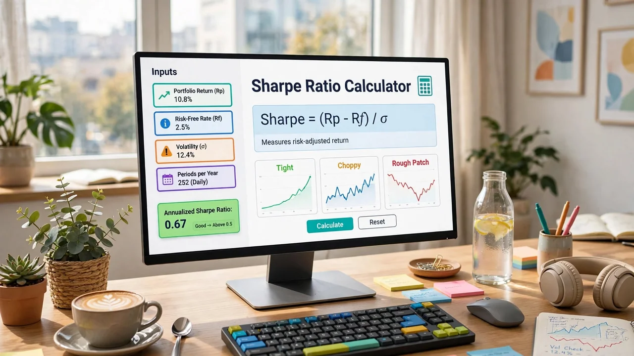
A ratio is a single number, and a single number hides the path that produced it. The three rows below are simulated series, illustrative only — not product results and not real accounts, each built to the same mean monthly return of 1.2000% so every curve reaches roughly the same place after twelve months. Only the dispersion changes, and that alone moves the ratio by a factor of four.
| Simulated curve | Monthly dispersion | Path shape | Annualised ratio (N=12) |
|---|---|---|---|
| A — tight | σ = 1.10% | Climbs in almost a straight line, month after month | 3.7788 |
| B — the worked example above | σ = 2.2529% | Visible chop quarter to quarter, no single bad stretch | 1.8451 |
| C — one rough patch | σ = 4.50% | Flat-to-up most months, then one sharp two-month give-back mid-year | 0.9237 |
End point: all three. Ratio: a factor of four apart. Curve C still finishes in the same place as A and B — the bad patch gets made back by year end — but the ratio is lower because the formula measures the bumpiness of the ride, not just where it ends. This is also why path matters separately from the ratio (more on that below): a reader looking only at the ending balance of A and C would call them equivalent, and the Sharpe ratio is the number that tells you they were not.
Reading the Number You Just Got
Threshold bands get quoted everywhere without the two facts that make them mean anything: the sampling frequency the figure was computed on, and how many observations went into it. A ratio quoted without both is not a comparable number. The bands below are the usual ones, each stamped with the conditions they assume.
| Annualised Sharpe | Common reading | Conditions it assumes |
|---|---|---|
| Below 0 | Lost to the risk-free baseline | Any frequency, any n — the sign is the one robust part |
| 0 to 1.0 | Weak to acceptable | Daily sampling, several hundred observations minimum |
| 1.0 to 2.0 | Good to institutional-grade | Daily sampling, multiple years, and a single pre-specified test |
| Above 2.0 | Rare | Treat as a prompt to re-check N, the sample length and how many variants were tried |
The best figure out of a long search is partly the search talking
Run one strategy and measure its ratio and the number means roughly what it says. Run a parameter sweep, take the best cell and the number now contains the sweep as well as the strategy — the more variants you tried, the further the winner sits above what it will repeat out of sample. Our own internal grids are explicit about this: one bounded structure sweep carried 396 effective tests and a haircut factor of 3.4587, meaning the selected cell's figure had to clear that multiple of its standard error before it counted as evidence of anything.
The formal correction is the deflated Sharpe ratio, which adjusts the figure for how many independent tests produced it. The Sharpe ratio glossary entry carries the definition, and overfitting in trading plus walk-forward testing cover what to do about it.
What the ratio cannot see
- Path. Standard deviation is order-blind. One brutal week buried inside an otherwise smooth year barely moves it, while that same week is what decides whether the strategy is still being traded. Read the ratio next to max drawdown, which is entirely about path.
- Fat tails. The denominator summarises dispersion as if returns were well behaved. Strategies that collect small premiums and occasionally give back a large one have exactly the return shape that makes a standard deviation flattering.
- Upside is penalised like downside. A big winning month raises dispersion and therefore lowers the ratio, which is arithmetically correct and economically odd. The Sortino ratio exists because of this; the glossary entry compares the two.
Where This Fits
A ratio is a measurement, and it is only as honest as the backtest underneath it. A backtest built on repainting signals overstates the mean and understates the dispersion, which flatters the numerator and the denominator at the same time. Quantzee's indicators are non-repainting, so the return series a Strategy Tester hands you is the one that was genuinely available in real time — which is the series this calculator assumes you are pasting in.
Also worth reading beside this number: the equity curve simulator and drawdown distribution, why profit factor flatters bad strategies, and the stress-testing checklist.
FAQ